K-Expectation Index 2.0: A Korean Stock Market Sentiment Index Built from 21 Indicators and 20 Years of KOSPI Data (Grade 9 Today)

Expectations are measured in money, not prices. The K-Expectation Index 2.0 is a Korean stock market sentiment index built from the numbers Korea publishes every day: investor deposits, margin loans, unpaid purchases, trading value, PBR, the VIX and USD/KRW. Like a credit rating model, it runs in five steps: item scores, a points table, a dispersion multiplier, the index and 10 grades. This report explains how it was tested on 20 years of data, how it did at six KOSPI peaks and eight bottoms, and why it reads 62.3, Grade 9, on October 13, 2026, with the KOSPI 33.8% below its June 22 peak.

• Of 21 candidate indicators, 10 worked in the same direction in both 2006-2014 and 2016-2026. Version 2.0 scores them (3-year percentiles, seven flipped), adds them at 10 points each (price 10, cash 20, debt 30, heat 20, fear 20) and applies a dispersion multiplier: 50 + (base score – 50) × (standard deviation of five domain scores ÷ 21.0).
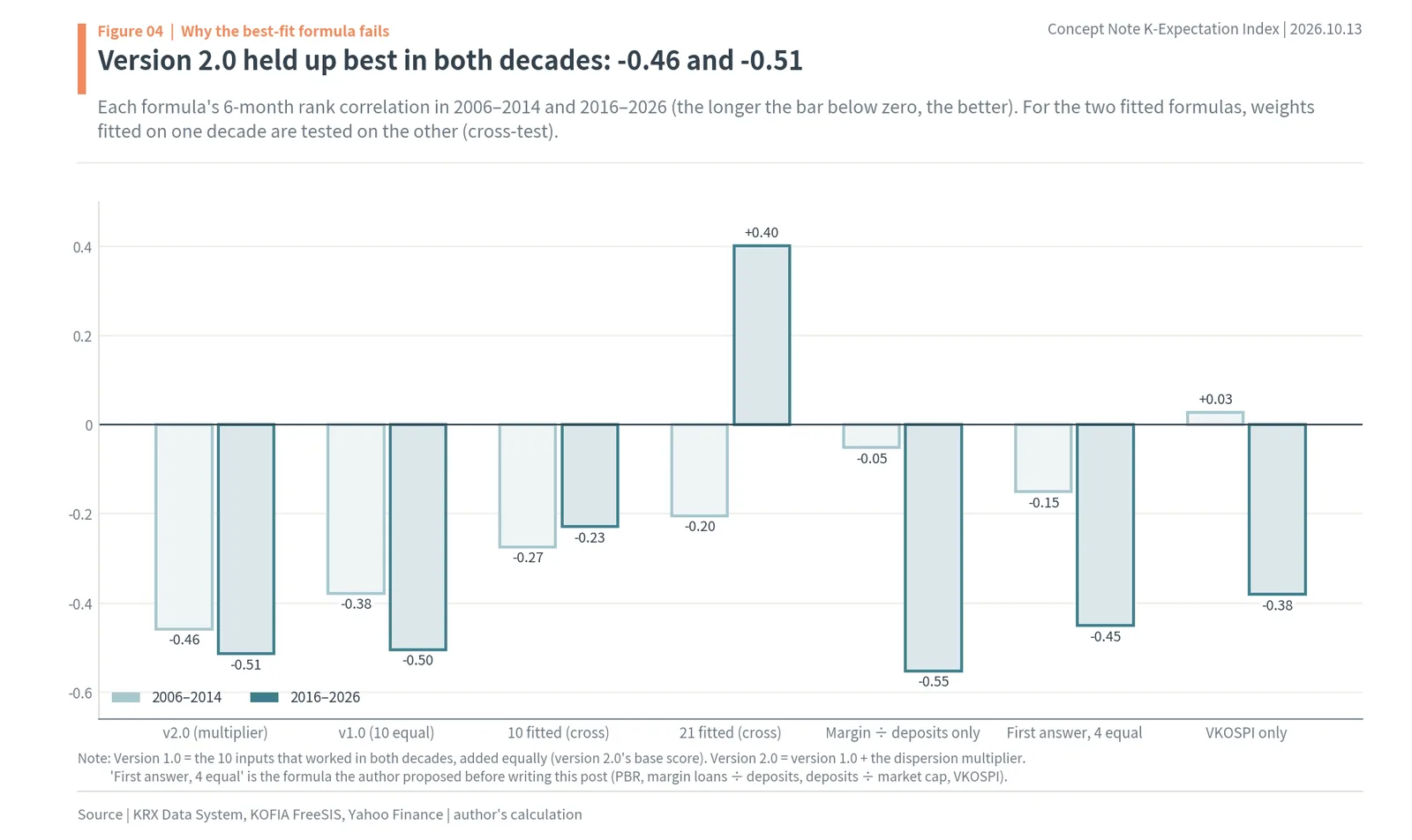
• Fitting the best weights to all 21 scored -0.46 on the past but +0.40 when fitted on the first decade and tested on the second; the equal-weight version 1.0 scored -0.38 and -0.50, and version 2.0 -0.46 and -0.51.
• Buying the KOSPI in Grade 1 (below 32.7) returned +29.4% on average six months later, with 96% of days up; Grade 10 (above 68.3), -4.8%, with 24% up; any day since 2006, +4.1%.
• At eight KOSPI bottoms since 2006 the index was 39.5 or lower (within Grade 2); at six peaks it was 47.6 or higher.
• Today: base score 73.8, domain standard deviation 10.8, multiplier 0.516, so the index is 62.3, Grade 9 (top 19.6%). Since June 22 investor deposits fell 24% to KRW 100.4tn (about $75.0bn) while margin loans fell only 11% to KRW 34.3tn.

Key takeaways

• The author tested 21 candidate indicators of Korean stock market expectations on 20 years of data, from 2006 to October 2026. Using the 10 that worked in the same direction in both 2006–2014 and 2016–2026 as inputs, he built the K-Expectation Index 2.0 the way a credit rating model is built: an item score table, a points table, a dispersion multiplier and a 10-grade table. Each device was kept only if it improved results in both decades.
• Buying the KOSPI in Grade 1 (below 32.7) returned an average of +29.4% six months later, and 96% of those days were up. Grade 10 (above 68.3) averaged -4.8%, with 24% up. Buying on any day since 2006 averaged +4.1%. The 6-month rank correlation improved from version 1.0, a simple average (-0.38 in the first decade, -0.50 in the second), to -0.46 and -0.51.
• On October 13, 2026 the KOSPI closed at 6,035.35, 33.8% below its June 22 peak, yet the index reads 62.3: Grade 9 of 10, at the threshold of the overheated zone. Since the peak, investor deposits have fallen 24% while margin loans fell only 11%; the won has strengthened and the US market is calm. The author reads today not as a bottom where expectations have broken, but as a stretch where the buyers are running out.

As of: October 13, 2026

Concepts covered: investor sentiment indicators, percentiles and rank correlation, 21 candidate indicators (PBR, PER, margin loans, unpaid purchases, investor deposits, turnover, trading value, VKOSPI, VIX, USD/KRW, forced selling, gap to the 120-day average, distance from the 52-week high, up-day ratio, flows by investor type), overfitting and the two-decade test, the K-Expectation Index 2.0 (item scores, points table, dispersion multiplier, 10 grades), devices tested and dropped, forward returns by grade, six peaks and eight bottoms, the 2026 KOSPI, today’s inputs, what it would take to reach a bottom grade, and how to calculate it yourself

Data: KOSPI and KOSDAQ index levels and market caps, trading value, VKOSPI, KOSPI PBR and PER, and trading by investor type come from the KRX Data System (closes through October 13, 2026). Investor deposits, margin loans, unpaid purchases and forced selling come from KOFIA FreeSIS (through October 12, published a day late). The US VIX and USD/KRW come from Yahoo Finance (October 13). KRX still showed the October 13 KOSPI PBR as 0, so it was estimated by applying the index change to the October 12 PBR. The photos are CC BY-SA photos from Wikimedia Commons. All index calculations are the author’s.

Summary: a Korean stock market sentiment index reads Grade 9 (62.3) even after a 33.8% KOSPI drop

This report asks one question. To actually use the old advice “buy when expectations have collapsed and sell when they run high” in the Korean stock market, what should expectations be measured with, and with what formula? The author gathered 21 candidate indicators and calculated their values for every day from January 2006 to October 2026. The test was a single one: the higher a day’s score, the lower the KOSPI return 3 months, 6 months and 1 year later should be.

The results come in four steps. First, putting all 21 indicators in and fitting the weights to work as well as possible on the past gave the best record on the past (a rank correlation of -0.46). But when the weights were fitted on the first decade only and tested on the second, the result was +0.40, the exact opposite. The formula had memorized the accidents of the past. Second, the author kept only the indicators that worked in the same direction in each decade, tested separately. Ten were left, and adding them at 10% each, version 1.0, worked in both periods: -0.38 in the first decade and -0.50 in the second. Third, he added, one at a time, devices commonly used in credit rating models: score curves, adjusted domain points, a crisis deduction and an overheating bonus. The only device that improved results in both decades was the “dispersion multiplier,” which strengthens the score according to how far the signals of the five domains diverge. Version 2.0, with the multiplier, scores -0.46 and -0.51. Fourth, when version 2.0 is split into 10 grades, Grade 1 returned +29.4% six months later (96% up) and Grade 10 returned -4.8% (24% up).

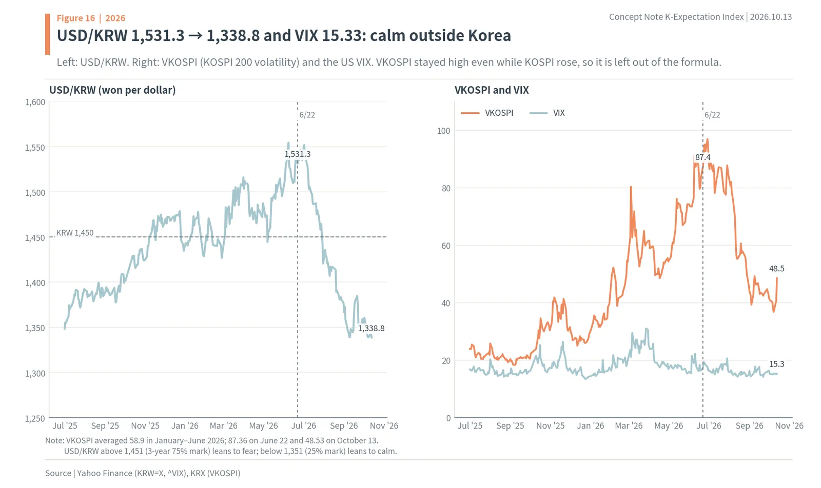
Today’s reading is 62.3, Grade 9. Although the KOSPI fell 33.8%, from 9,114.55 on June 22 to 6,035.35 on October 13, the index is higher than on June 22 (51.4). Investor deposits fell 24%, from KRW 132.2tn (about $98.7bn) on June 22 to KRW 100.4tn (about $75.0bn) on October 12, while margin loans fell only 11%, from KRW 38.5tn to KRW 34.3tn (about $25.6bn). The money to buy with is leaving, but the debt is still there. USD/KRW came down from 1,531.3 on June 22 to 1,338.8, so the won has strengthened, and the US VIX at 15.33 says the market outside Korea is calm. The 20-day average trading value of KRW 29.1tn is below two-thirds of the 120-day average of KRW 44.8tn, so there has been no capitulation-style surge in trading either. All five domains are evenly high, so the dispersion multiplier (0.516) pressed the base score of 73.8 down to 62.3, but the index is still at the threshold of the overheated zone.

The author reads today not as a bottom where expectations have broken, but as a stretch where the buyers are running out. By the author’s calculation, if prices fall another 20% with everything else unchanged, the index is 58.2 (Grade 8). Only if a 20% price drop comes with a quarter of margin debt cleared, the US VIX at 35 and USD/KRW at 1,450 does it come down to 43.0 (Grade 3), and it takes the same capitulation plus money flowing back into deposits to reach the Grade 2 threshold (39.8). This report walks through how it gets to that conclusion, in this order: how to measure expectations, the 21 candidates, the overfitting trap, the 2.0 formula, the grade report card, peaks and bottoms, 2026, today’s inputs, the conditions for a bottom, how to calculate the index yourself, and the calculation basis.

How it works in Korea: daily investor deposits, margin loans and flows from KOFIA and KRX

A sentiment index built for Korea can use data that most markets do not publish. Three Korea-specific facts make the K-Expectation Index possible.

First, the money waiting on the sidelines and the money borrowed to buy stocks are published every trading day. The Korea Financial Investment Association (KOFIA), the industry body for brokers and asset managers, posts daily figures on its FreeSIS statistics site for investor deposits (cash parked in brokerage accounts to buy stocks), margin loans (money borrowed from brokers to buy stocks), unpaid purchases (money owed for shares bought but not paid for by the settlement date) and forced selling (positions a broker sells off when an investor’s collateral falls short). The figures come out one day late, so today’s index uses yesterday’s KOFIA numbers.

Second, the Korea Exchange (KRX) publishes net buying by investor type, foreigners, individuals (retail) and institutions, every day. So who bought and who sold is a matter of record. This report tested those flows as candidates, although none of them made the final formula.

Third, the market has two boards. The KOSPI is the main board of the Korea Exchange and its benchmark index; the KOSDAQ is the exchange’s growth market, home to smaller tech and biotech companies. The index uses the combined market cap and trading value of both boards, since KOFIA’s deposit and margin loan totals cover both. The VKOSPI is the KRX’s implied-volatility index for the KOSPI 200, the Korean counterpart of the VIX. The exchange rate matters too: when the won weakens (USD/KRW rises), foreign investors often sell Korean stocks.

Korea counts large sums in units of jo, or one trillion won. This report writes them as KRW tn: KRW 1tn is about $747mn. Dollar figures use KRW 1,338.76 per dollar, the October 13, 2026 rate (Yahoo Finance).

How to measure market sentiment: percentiles, expectation scores and rank correlation

Expectations are the optimism in prices plus the ammunition left

When people say expectations are high in the stock market, they mean two things at once. One is that a lot of optimism about good things to come is already in the price. The other is that, because of that optimism, the buyers have already bought, so not much money is left to buy more. That is why on days when expectations run high, good news struggles to lift prices further, and a small disappointment shakes them hard. On days when expectations have collapsed, the price already holds a lot of pessimism, and the money of those who sold in fear sits in their accounts. Bad news then hurts less, and good news gets a big reaction. This is why “buy when expectations have collapsed and sell when they run high” works.

The problem is that there is no ruler that measures expectations directly. The US has indexes that blend several indicators, such as CNN’s Fear & Greed Index, but the Korean market is built differently: retail investors’ debt (margin loans) and cash (investor deposits) are published every day, and the exchange rate drives foreign trading. So the author gathered indicators among the numbers published daily in Korea that could show expectations, and tested on 20 years of data which of them actually moved against future prices.

Putting indicators with different units on one percentile scale

The candidates come in different units. PBR is 1.50x, margin loans ÷ deposits is 34.1%, USD/KRW is 1,338.8 and the VIX is 15.33. These cannot simply be added up. So every indicator was converted into how high today’s value ranks within the prior 3 years (756 trading days). This is its percentile. A percentile of 80 means today’s value is higher than on 80% of the days in the prior 3 years; 100 means it is the highest of the 3 years. This turns every indicator into a score between 0 and 100 that can be added and compared.

There are two reasons for a 3-year window. The big swings in the Korean market tend to change every 2 to 4 years, so 3 years usually holds one rise and one fall. A 3-year window also reduces the problem of indicators growing or shrinking over the decades. Investor deposits, for example, went from the KRW 10tn range in 2006 to the KRW 100tn range in 2026. Raw amounts would always read “high” in recent years, but a rank within the prior 3 years shows whether a value is high or low for its own era.

Turning percentiles into expectation scores

Some indicators move with expectations and some move against them. A higher PBR means more optimism in the price, so it is used as is. A higher VIX, on the other hand, means more fear, which is the opposite of expectations. So for indicators like the VIX, the score is 100 minus the percentile. This report calls the direction-adjusted score the “expectation score.” For every input, a higher expectation score points to higher expectations, that is, to weaker returns ahead.

The data, not the author, set each direction. If returns were weaker after an indicator was high, it was used as is; if returns were stronger after it was high, it was flipped. As a result some inputs go in the opposite direction from common sense. For example, returns were actually better after margin loans grew fast. Growing debt means buyers are still coming in. These inputs are explained one by one in the formula section below.

Rank correlation as the test

If a formula measures expectations well, then the higher its score on a given day, the lower the later return should be. The strength of that relationship was measured with rank correlation. Rank correlation converts two sets of numbers into rankings and measures, on a scale from -1 to +1, how closely the rankings move together. If later returns are lower on days with higher scores, it is close to -1; if there is no relationship, 0; if it is the other way around, close to +1. Because it works on ranks, one or two big moves such as 2008 or 2020 do not dominate the result. In data as noisy as stock returns, a rank correlation of -0.3 is a fairly useful relationship and -0.5 is a strong one.

Later returns were measured over three horizons together: 3 months (60 trading days), 6 months (120 trading days) and 1 year (250 trading days). Fitting a single horizon tends to pick a formula that works on that horizon by accident. To choose formulas, the three horizons’ returns were scaled to the same size and averaged into one target; to present results, the report centers on 6 months, the easiest to read. Once the inputs are chosen, what remains is how to combine their scores into one index. Like a credit rating model, this report uses five steps: an item score table that scores each input, a points table that sets how many points each domain gets, a dispersion multiplier that strengthens or weakens the score according to how far the domains’ signals diverge, the index calculation that combines these three, and a grade table that splits the final score into 10 grades. Each grade comes with a report card of what happened after buying in that grade in the past. Every device was kept only if it passed the two-decade test. The result is the K-Expectation Index 2.0, and its October 13 value is 62.3, Grade 9 of 10. Figure 1 shows Yeouido in Seoul, where Korea’s brokerages are clustered. Every input to this index is a number about the money that moves through here.

Testing in two separate decades

The most important device is splitting the period in two: 2006–2014 (the first decade) and 2016–2026 (the second decade), with 2015 left empty so the later returns of the two periods do not overlap. The first decade held the 2008 global financial crisis, the 2011 European debt crisis and the long range-bound market that followed. The second held the 2018 chip peak, COVID-19 in 2020, the 2021 “Donghak ant” retail buying wave and the 2025–2026 memory chip surge. An indicator that worked in the same direction in two periods with such different markets is unlikely to be an accident. This is the yardstick this report uses to define “best.”

21 candidate sentiment indicators: price, debt, cash, heat, fear, trend and flows

Price, debt, cash, heat, fear, trend and flows

The candidates were chosen from numbers that are published daily in Korea, have records going back before 2006, and could show investors’ optimism or ammunition. There are 21 in all, in seven groups.

The price group looks at how expensive stocks are relative to earnings and assets. It has two indicators: KOSPI PBR (price ÷ book value per share) and PER (price ÷ earnings per share over the past year). KRX calculates both for the KOSPI as a whole, as if it were one company, and publishes them daily. When more optimism goes into prices, investors pay more for the same earnings and assets, so PBR and PER rise.

The debt group looks at how much retail investors bought with borrowed money. It has four indicators: margin loans ÷ investor deposits; margin loans ÷ KOSPI and KOSDAQ market cap; the 5-day average of unpaid purchases ÷ deposits; and margin loan growth, the percentage change in margin loans over 60 trading days. Debt measures the size of optimism, and it is also what makes selling cascade through forced liquidations when prices fall. The amounts have changed enormously. KOFIA data put margin loans at an average of KRW 0.5tn in 2006 and KRW 34.3tn on October 12, 2026.

The cash group looks at how much money is left to buy stocks. It has two indicators: investor deposits ÷ market cap, and deposit growth, the percentage change in deposits over 60 trading days. Deposits grew from an average of KRW 10.9tn in 2006 to KRW 139.7tn (about $104.4bn) on June 4, 2026.

The heat group looks at how hot trading is. It has three indicators: turnover, the 20-day average trading value (KOSPI plus KOSDAQ) ÷ deposits; trading surge, the 20-day average trading value ÷ the 120-day average; and KOSDAQ relative strength, the KOSDAQ’s 60-day return minus the KOSPI’s. KOSDAQ relative strength was included to capture the speculative heat of retail investors crowding into small stocks.

The fear group looks at how scared investors are. It has four indicators: the VKOSPI, the expected 30-day volatility backed out of KOSPI 200 option prices; the VIX, the same measure from the US S&P 500; USD/KRW; and forced selling, the 5-day amount of forced selling ÷ deposits. USD/KRW is in the fear group because when it rises (when the won weakens), foreign investors often sell Korean stocks and leave.

The trend group looks at how far prices have run. It has three indicators: the gap to the 120-day average (KOSPI ÷ its 120-day moving average), the distance from the 52-week high, and the up-day ratio, the share of up days in the last 10 trading days. The flows group has three indicators: the net buying of foreigners, retail and institutions in the KOSPI over 20 trading days, each divided by KOSPI market cap.

Testing one by one: half changed direction from one decade to the next

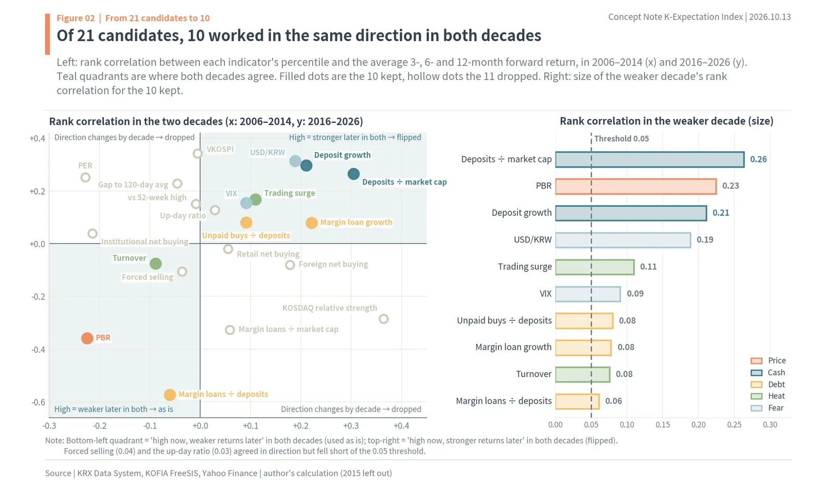
All 21 were tested one at a time. In Figure 2, the horizontal axis is the rank correlation in the first decade (2006–2014) and the vertical axis is the rank correlation in the second decade (2016–2026). Here the rank correlation is between each indicator’s percentile (before any flipping) and the average of its 3-, 6- and 12-month later returns. A dot in the bottom-left quadrant means “returns were weaker after it was high” in both decades; a dot in the top-right quadrant means “returns were stronger after it was high” in both decades. Both quadrants point the same way in both decades, so both can be used: indicators in the top-right quadrant simply go in flipped. Indicators in the top-left or bottom-right quadrants worked in one decade and went the other way in the other.

The most dramatic case is KOSDAQ relative strength. In the first decade it was +0.36, meaning returns were better after the KOSDAQ outperformed the KOSPI; in the second decade it was -0.28, the opposite. PER also changed direction, at -0.23 in the first decade and +0.25 in the second. PER, calculated on the past year’s earnings, reads high early in an earnings upswing and low as earnings approach their peak. In the second decade, with its big swings in chip earnings, this property flipped PER’s direction. The KOSPI’s PER fell 57%, from 24.8x on June 22, 2026 to 10.64x on October 12, while its PBR fell 39%, from 2.59x to 1.59x over the same period. The difference is how much earnings grew.

The VKOSPI was -0.01 in the first decade, almost no relationship, and +0.34 only in the second. In 2008 the VKOSPI jumped to 62.7 in the second week of October, and even after that the KOSPI fell further, from 1,241 to 938.75 on October 24. In 2026, daily swings stayed large even while the KOSPI rose, keeping the VKOSPI high. On June 22, 2026, the day of the KOSPI’s peak, the VKOSPI was 87.36. It was high not because of fear but because the market was swinging hard in both directions. The gap to the 120-day average and the distance from the 52-week high were also clear only in the second decade, and net buying by foreigners, retail and institutions was weak or changed direction in both decades.

Some indicators, by contrast, held the same direction steadily in both decades. Deposits ÷ market cap was the steadiest, at +0.31 in the first decade and +0.26 in the second. When deposits were large relative to market cap, that is, when a lot of buying money was still left, later returns were good. PBR was -0.23 and -0.36, USD/KRW +0.19 and +0.31, and deposit growth +0.21 and +0.30. Margin loans ÷ deposits was -0.57 in the second decade, the strongest of the 21, but only -0.06 in the first decade, because margin lending itself was small in 2006–2014.

The ten that remained

The indicators kept were those with the same direction in both decades and a rank correlation of at least 0.05 in size in the weaker decade. The 0.05 bar is a minimum threshold to make sure that “same direction” is not just noise. Ten indicators cleared it: deposits ÷ market cap, PBR, deposit growth, USD/KRW, trading surge, VIX, unpaid purchases ÷ deposits, margin loan growth, turnover, and margin loans ÷ deposits. Forced selling (0.04 in the weaker decade) and the up-day ratio (0.03) had the same direction but missed the threshold. By group, the ten break down into one price input (PBR), two cash inputs (deposits ÷ market cap, deposit growth), three debt inputs (margin loans ÷ deposits, unpaid purchases ÷ deposits, margin loan growth), two heat inputs (turnover, trading surge) and two fear inputs (VIX, USD/KRW). Nothing from the trend or flows groups survived.

Overfitting: the 21-indicator best fit scored +0.40 in a decade it had not seen

Fitting the best weights to all 21

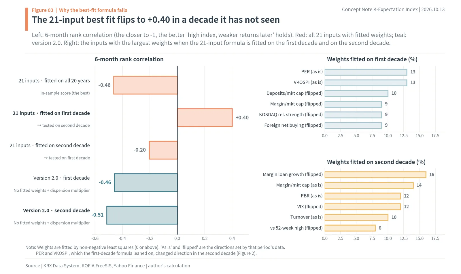
The first thing tried was to put all 21 in and find the weights that fit the past best. The method was non-negative least squares. After setting each indicator’s direction from the data, it chooses non-negative weights for the expectation scores so that their weighted sum moves as closely as possible against the 3-, 6- and 12-month later returns. Keeping the weights at zero or above means useless indicators get a weight of zero and drop out on their own. Run on all of 2006–2026, this left 13 of the 21, with a 6-month rank correlation of -0.46, higher than any other formula tested in this report. Splitting the score into five bins, the lowest 20% averaged +20.6% six months later and the highest 20% -5.2%. On the numbers alone, this is the “best formula.”

Fitted on the first decade, tested on the second: +0.40

But this formula has a trap. Its weights were set after seeing all the data through 2026, so there is no way to know whether they will hold in the future. The way to check is to set the weights on one period only and test them on the other. When the same calculation was run on 2006–2014 data alone and the resulting weights were applied to 2016–2026, the 6-month rank correlation was +0.40. Returns were actually higher after high scores. A formula built to measure expectations got it exactly backwards in a decade it had not seen. The other way around, a formula fitted on 2016–2026 and applied to 2006–2014 scored -0.20: the right direction, but less than half the strength.

Why this happens becomes clear when the two formulas’ weights are put side by side. The right side of Figure 3 compares the inputs with the largest weights in the formula fitted on the first decade and the one fitted on the second. The first-decade formula leaned on PER (13%), VKOSPI (13%), deposits ÷ market cap (10%), and KOSDAQ relative strength and foreign net buying (9% each). PER and VKOSPI went in with the “high now, weaker returns later” direction in the first decade, and as shown earlier, both changed direction in the second. The second-decade formula leaned on margin loan growth (16%), margin loans ÷ market cap (14%), and PBR and the VIX (12% each). The inputs the two formulas considered important barely overlap. When as many as 21 inputs are used to explain one period’s ups and downs as fully as possible, the weights absorb even the accidental relationships that existed only in that period. Statisticians call this overfitting. It is like a student who memorized the answers to past exams and falls apart on a new one.

Choosing inputs from one decade also weakens results

The same problem arises even without fitting weights, just by choosing inputs. Within the first decade, the author split the data again into two 5-year halves, picked the inputs with the same direction in both halves and added them equally. The inputs chosen were PBR, PER, margin loans ÷ deposits, deposits ÷ market cap, turnover, KOSDAQ relative strength and USD/KRW. Applied to the second decade, this formula had a 6-month rank correlation of -0.17: the right direction, but weak. Doing the same on the second decade and applying it to the first gave -0.15. The two halves within one decade have a similar market character, so agreeing in direction there is no guarantee of working in a different era. That is why this report required inputs to point the same way in two decades from different eras.

The other formulas, side by side in both decades

Figure 4 lines up the formulas tested in this report by their 6-month rank correlation in the first and second decades. The final formula, the K-Expectation Index 2.0, scores -0.46 in the first decade and -0.51 in the second. Its foundation, version 1.0 (the ten inputs that worked in both decades, added equally), scores -0.38 and -0.50. The only thing version 2.0 adds to version 1.0 is the dispersion multiplier, explained in the next section. A formula with the same ten inputs but weights fitted to the data looks similar over the full period, at -0.34 and -0.53, but weights fitted on the first decade score -0.23 on the second, and weights fitted on the second score -0.27 on the first, weaker than the equal-weight formula. Fitting weights itself invites accidents. So version 2.0 also does not fit input weights and gives each input an equal 10%.

Single-indicator formulas were compared too. Margin loans ÷ deposits alone was strong in the second decade at -0.55, but barely worked in the first, at -0.05. The VKOSPI alone, flipped (treating more fear as lower expectations), scored +0.03 in the first decade and -0.38 in the second. The formula the author first proposed before writing this report, four inputs (PBR, margin loans ÷ deposits, deposits ÷ market cap, VKOSPI) added equally, scored -0.15 and -0.45. None held up in both decades as well as version 2.0.

So the meaning of “best” changed

The conclusion of this section is that the standard for the “best formula” has to change. A formula that fits the past 20 years best can always be built; the more inputs and the finer the weights, the better the past record. But what someone using this index needs is not a formula that explains the past; it is one that works on days that have not come yet. So in this report, “best” means a formula that works in a decade it has not seen. On that condition the inputs were chosen (the ten that worked in both decades), the weights were left unfitted, and only adjustments that improved results in both decades were added. Over the full period, version 2.0’s rank correlation is -0.44 at 6 months, -0.34 at 3 months and -0.50 at 1 year, almost the same as or better than the 21-input best fit (-0.46, -0.39 and -0.48). The choice gives up almost nothing on the past record and does not fall apart in a period it has not seen.

The K-Expectation Index 2.0 formula: item scores, points table, dispersion multiplier and 10 grades

A formula in five steps

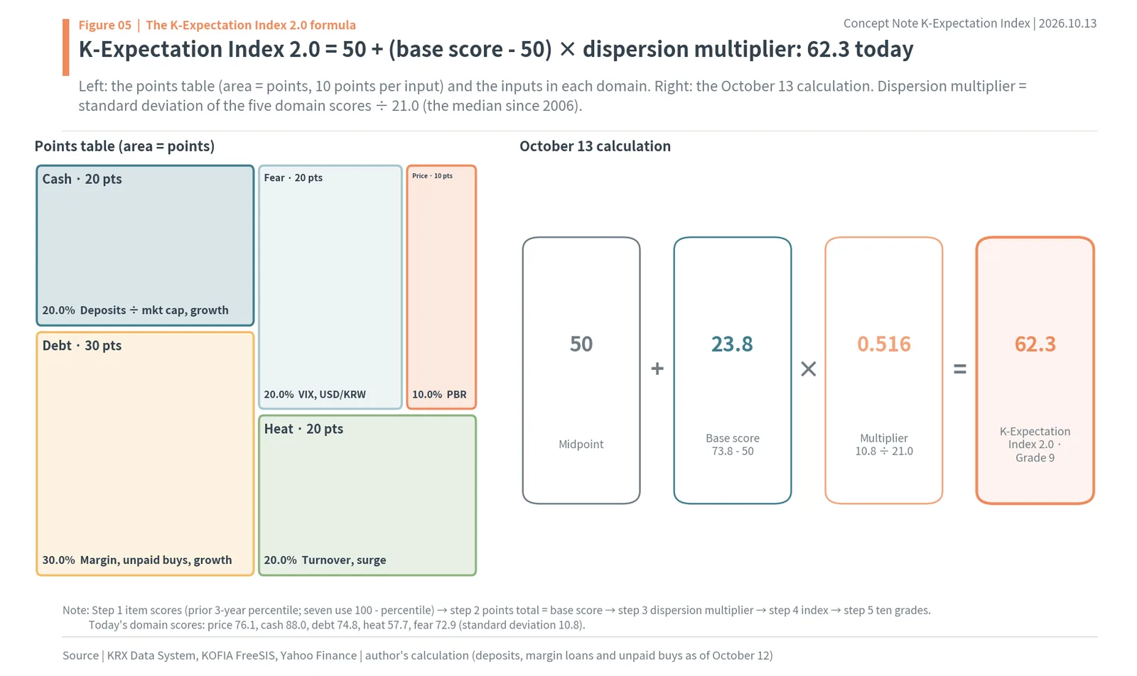
The K-Expectation Index 2.0 is calculated in five steps, like a credit rating model. Step 1 is the item score table. Each of the ten inputs is converted into its percentile within the prior 3 years (756 trading days), and for the seven after which high values were followed by better returns, the percentile is subtracted from 100. This makes all ten into 0-to-100 scores that point the same way: the higher, the higher the expectations. Step 2 is the points table. The ten scores are added at 10% each to give the base score. Grouped by domain, that is price 10 points, cash 20, debt 30, heat 20 and fear 20, for 100 points in total. Step 3 is the dispersion multiplier. It measures how spread out the five domain scores (the average score of the inputs in each domain) are, as a standard deviation, and divides that by 21.0, the median since 2006. Step 4 calculates K-Expectation Index = 50 + (base score – 50) × dispersion multiplier, clipped to the ends if it falls outside 0 to 100. Step 5 is the grade table. The index values since 2006 are sorted by size into ten equal bins, from Grade 1 (below 32.7) to Grade 10 (above 68.3).

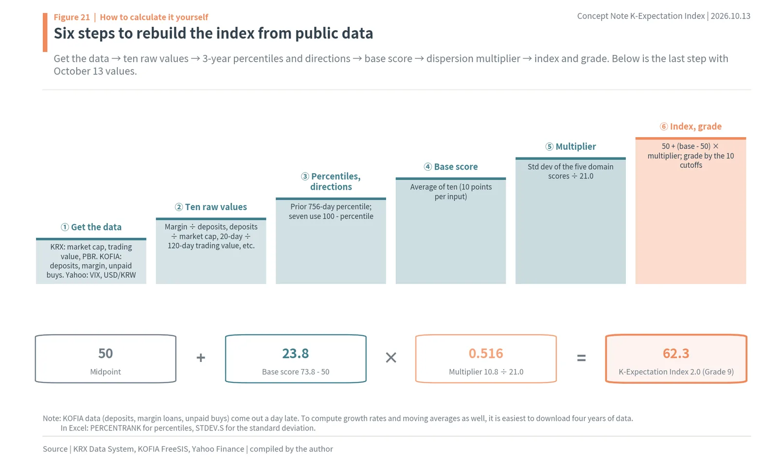
Here is how it works with October 13 values. The ten expectation scores add up to 737.6, so the base score is 73.8. The five domain scores are price 76.1, cash 88.0, debt 74.8, heat 57.7 and fear 72.9, and the standard deviation of these five values is 10.8. The dispersion multiplier is 10.8 ÷ 21.0 = 0.516. The base score is 23.8 above 50, so 50 + 23.8 × 0.516 = 62.3 is the K-Expectation Index 2.0. By the grade cutoffs, it falls between 62.0 and 68.3, so it is Grade 9. The left side of Figure 5 is the points table; the right side writes the calculation as an equation.

The ten inputs and their directions

The ten inputs and their directions are as follows. Price is KOSPI PBR (as is). Cash is deposits ÷ KOSPI and KOSDAQ market cap (flipped) and 60-trading-day deposit growth (flipped). Debt is margin loans ÷ deposits (as is), the 5-day average of unpaid purchases ÷ deposits (flipped) and 60-trading-day margin loan growth (flipped). Heat is 20-day average trading value ÷ deposits (as is) and 20-day ÷ 120-day average trading value (flipped). Fear is the US VIX (flipped) and USD/KRW (flipped). The debt domain gets the most points, 30, not because the author chose it, but because three of the inputs that passed the two-decade test came from the debt group.

The three inputs used as is follow intuition. The higher PBR is, the more optimism is in the price, and its rank correlation with 1-year later returns was -0.37 (-0.31 in the first decade, -0.42 in the second). A high margin loans ÷ deposits ratio means investors carry a lot of debt relative to their cash, and when prices fall, forced selling deepens the decline. High turnover (20-day average trading value ÷ deposits) means more day trading and chasing with the same cash.

Of the seven flipped inputs, four are about buying power and fear outside Korea. When deposits are large relative to market cap, a lot of cash that has not yet bought stocks is still waiting and has the power to push prices up; when deposits are growing, new money is coming in. These two inputs were the steadiest across both decades of all 21 (rank correlations of 0.26 and 0.21 in their weaker decade). A high VIX or a high USD/KRW (a weak won) means investors are scared, and KOSPI bought at such times did well later. USD/KRW had a rank correlation of +0.34 with 1-year later returns. The remaining three go in against intuition. With margin loan growth, returns were actually better after debt grew fast. A high level of debt is bad, but the fact that debt is growing signals that buyers are still coming in. With unpaid purchases ÷ deposits, returns were better after unpaid purchases were high. Unpaid purchases often build up when prices drop sharply and investors cannot settle, so they read as a sign that capitulation is already under way. With trading surge, returns were also better after trading suddenly piled up. A surge in trading shows up both when panic selling makes a bottom and when a new rally starts.

Why equal weights

As shown earlier, even with the same ten inputs, weights fitted to the data lost strength in the decade they had not seen (-0.23 and -0.27). Changing the points at the domain level was tested too. Giving each of the five domains an equal 20 points scored -0.35 in the first decade and -0.47 in the second, and giving each domain points in proportion to its weaker-decade rank correlation scored -0.35 and -0.46. Both were weaker than version 1.0, which gives each input 10% (-0.38, -0.50). Even with 20 years of data, there are only about 40 non-overlapping windows of 6-month returns. Fitting points precisely to that many observations means fitting noise too. So version 2.0 kept the simplest scheme: 10 points per input, so that the number of inputs in a domain is that domain’s points.

Where the dispersion multiplier came from

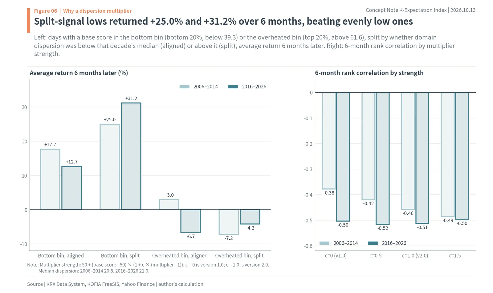
The one device version 2.0 adds to version 1.0 is the dispersion multiplier. It starts from a fact: at the same base score, later returns differed between days when the five domains spoke with one voice and days when they diverged. Figure 6 takes days when the base score was in the bottom 20% (below 39.3) or the top 20% (above 61.6) and splits them into days when the standard deviation of the domain scores was below that decade’s median (aligned) and above it (split), then looks at the return 6 months later. Among bottom-20% days, split days returned +25.0% in the first decade (93% up) and +31.2% in the second (96% up). Days when the domains were evenly low returned +17.7% and +12.7%. In both decades, the bottom signal was stronger on split days. Among top-20% days, split days returned -7.2% in the first decade (21% up) and -4.2% in the second (17% up), poor in both decades.

Put plainly, the signal is stronger on days when one or two domains swing to an extreme than on days when all five are each a little high or a little low. At a bottom, for example, that is a day when price is not yet very cheap but cash has piled up and fear has spiked; on the peak side, it is a day when price is not very expensive but cash has run dry and debt has piled up. The dispersion multiplier puts this difference into the formula. When the domains lean evenly and the dispersion is small, the multiplier drops below 1 and pulls the index toward 50; when only a few domains are extreme and the dispersion is large, the multiplier rises above 1 and pushes the index further from 50.

Adding the multiplier improved the 6-month rank correlation in both periods, from -0.38 to -0.46 in the first decade and from -0.50 to -0.51 in the second. The multiplier’s strength was tested too. Applying only half of the move from 1 to the dispersion multiplier gave -0.42 in the first decade and -0.52 in the second; applying it in full gave -0.46 and -0.51; strengthening it to 1.5 times gave -0.49 and -0.50. The first decade improved the stronger it got, while the second decade was best between half and full strength. The author used full strength (1.0), which satisfies both decades together.

Devices tested and dropped

Devices that commonly appear in institutional rating models were tested as well. Any device that did not beat version 1.0 in both decades was left out. First, score curves. Curves that compress the middle and stretch the ends (1.5th, 2nd and 3rd powers), a curve that does the opposite (0.6th power), and a step score table that gives 0, 2, 4, 5, 6, 8 or 10 points by band all scored -0.36 to -0.38 in the first decade and -0.48 to -0.50 in the second, the same as or weaker than version 1.0 (-0.38, -0.50). Second, a crisis deduction. On “fear peak” days, when the VIX and USD/KRW were both in the top 15% of the prior 3 years, the 6-month return within the same score bin was 13.1 percentage points higher in the first decade and 3.2 points higher in the second. But deducting 10 points on those days actually weakened the rank correlation, to -0.36 and -0.50, because fear-peak days already score low on the base score. Third, an overheating bonus and other combined signals. “Debt and trading overheating together” (margin loans ÷ deposits in the top 15% and turnover in the top 25%) scored +2.5 points in the first decade and -6.6 points in the second, a change of direction, and “debt fatigue” (high margin loans ÷ deposits but margin growth stalled) also changed direction, at -11.5 and +1.9 points. Signals that point in different directions in the two decades were left out of the formula.

KOSPI returns by sentiment grade: Grade 1 +29.4%, Grade 10 -4.8% six months later

Report card for ten grades

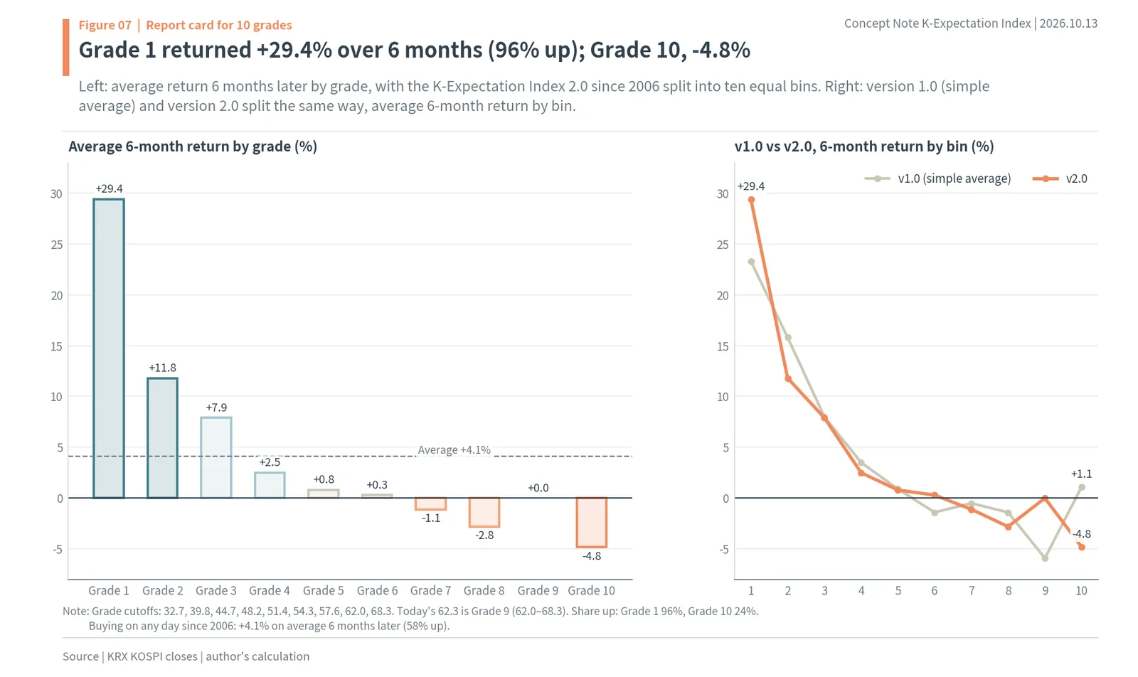
The grade table sorts every daily value of the K-Expectation Index 2.0 from January 2006 to October 2026 by size into ten equal bins. The cutoffs are 32.7, 39.8, 44.7, 48.2, 51.4, 54.3, 57.6, 62.0 and 68.3. Just as credit ratings come with the actual default rate for each grade, Figure 7 is a report card that attaches to each grade the average KOSPI return 6 months after buying on those days, and the share of those days that were up.

Days bought in Grade 1 (below 32.7) returned an average of +15.2% after 3 months (93% up), +29.4% after 6 months (96%) and +49.6% after 1 year (97%). Grade 2 (32.7 to 39.8) returned +11.8% after 6 months (74% up), Grade 3 +7.9% (72%) and Grade 4 +2.5% (62%). Grades 5 to 7 were near zero after 6 months, at +0.8%, +0.3% and -1.1%. Grade 8 returned -2.8% (43% up), Grade 9 0.0% (47%) and Grade 10 (above 68.3) -4.8% (24%), and Grade 10’s 1-year average was -11.4% (31% up). Buying on any day since 2006 averaged +1.9% at 3 months, +4.1% at 6 months (58% up) and +7.7% at 1 year. Grades 1 to 4 beat the average, and Grades 7 to 10 fell short of it.

Compared with version 1.0, the difference is largest at the top. Split the same way into ten bins, version 1.0, the simple average, had a top 10% that averaged +1.1% six months later: it could not pick out overheating. Version 2.0’s Grade 10 returned -4.8%, because days when the domains were merely evenly high were pulled toward 50 and out of the top bin.

Grouped into five zones

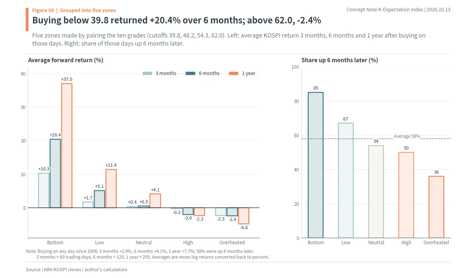
Pairing the ten grades into five zones makes the index easier to read. Grades 1 and 2 (below 39.8) are called the “bottom zone,” Grades 3 and 4 “low,” Grades 5 and 6 “neutral,” Grades 7 and 8 “high,” and Grades 9 and 10 (above 62.0) “overheated.” Figure 8 shows the average return after 3 months, 6 months and 1 year and the share of days up after 6 months in each zone. Days bought in the bottom zone returned +10.3% after 3 months (85% up), +20.4% after 6 months (85%) and +37.0% after 1 year (92%). The low zone returned +5.1% after 6 months (67% up), neutral +0.5% (54%), high -2.0% (50%) and overheated -2.4% (36%), and the overheated zone’s 1-year average was -4.8%. The higher the zone, the lower the later return, step by step. This staircase is the most direct evidence that the index measures expectations.

The index since 2006

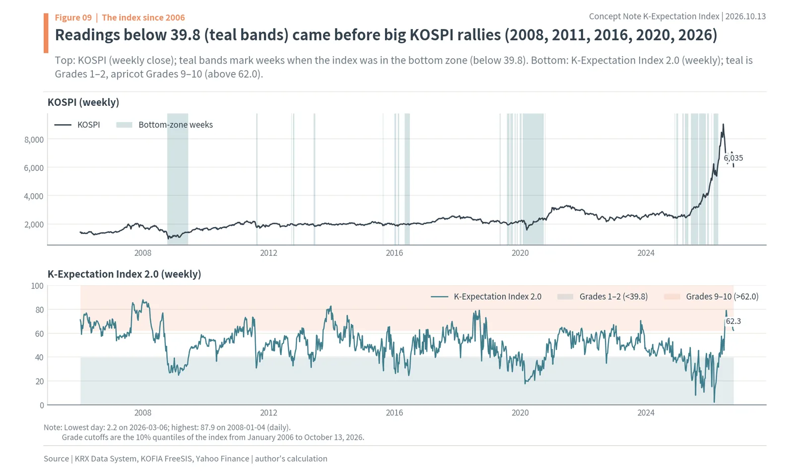
Figure 9 plots the KOSPI and the K-Expectation Index 2.0 weekly since 2006. The top panel is the KOSPI, with teal bands on the weeks when the index was in the bottom zone (below 39.8). The bottom panel is the index itself. The teal bands cluster in October 2008 to June 2009, August 2011, the first half of 2016, August 2019 to autumn 2020, and repeatedly between December 2024 and April 2026. Each was followed by a big KOSPI rise. The lowest day in 20 years was March 6, 2026 (2.2) and the highest was January 4, 2008 (87.9). On March 6, 2026 the KOSPI was at 5,584.87, and it rose 63.2% to 9,114.55 by June 22. January 4, 2008 was just as the first decline after the October 2007 peak was starting, and the KOSPI fell to 938.75 that October.

The same staircase within each decade

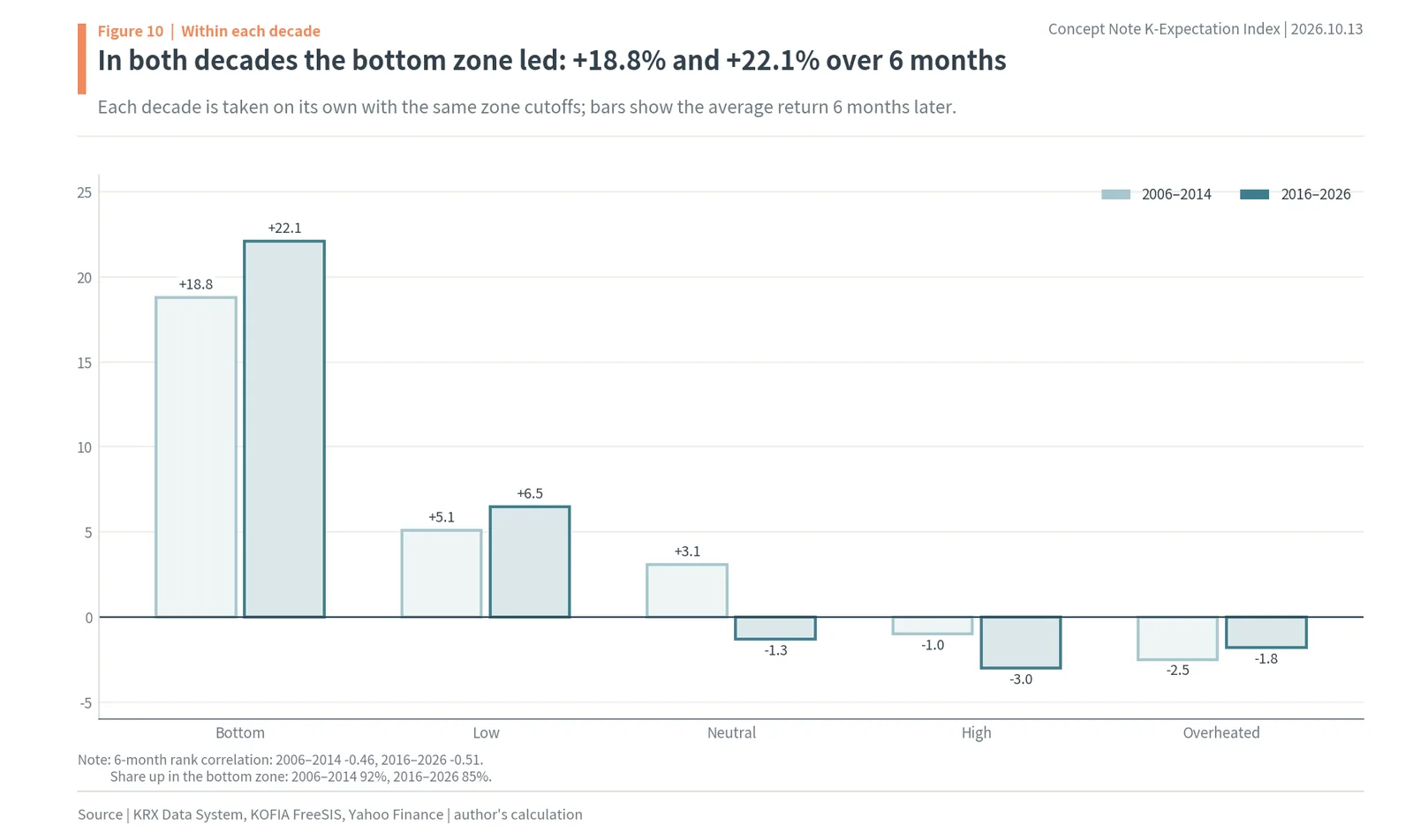
Results over the full period could be pulled along by the big bull markets of the second decade. So the two decades were looked at separately with the same zone cutoffs (Figure 10). In the first decade (2006–2014), days bought in the bottom zone averaged +18.8% six months later (92% up), low +5.1% (80%), neutral +3.1% (69%), high -1.0% (57%) and overheated -2.5% (37%). In the second decade (2016–2026), the figures were +22.1% (85%), +6.5% (66%), -1.3% (45%), -3.0% (44%) and -1.8% (34%). In both periods the bottom zone is far ahead, and returns fall as the zones rise. The 6-month rank correlation is -0.46 in the first decade and -0.51 in the second.

Week by week

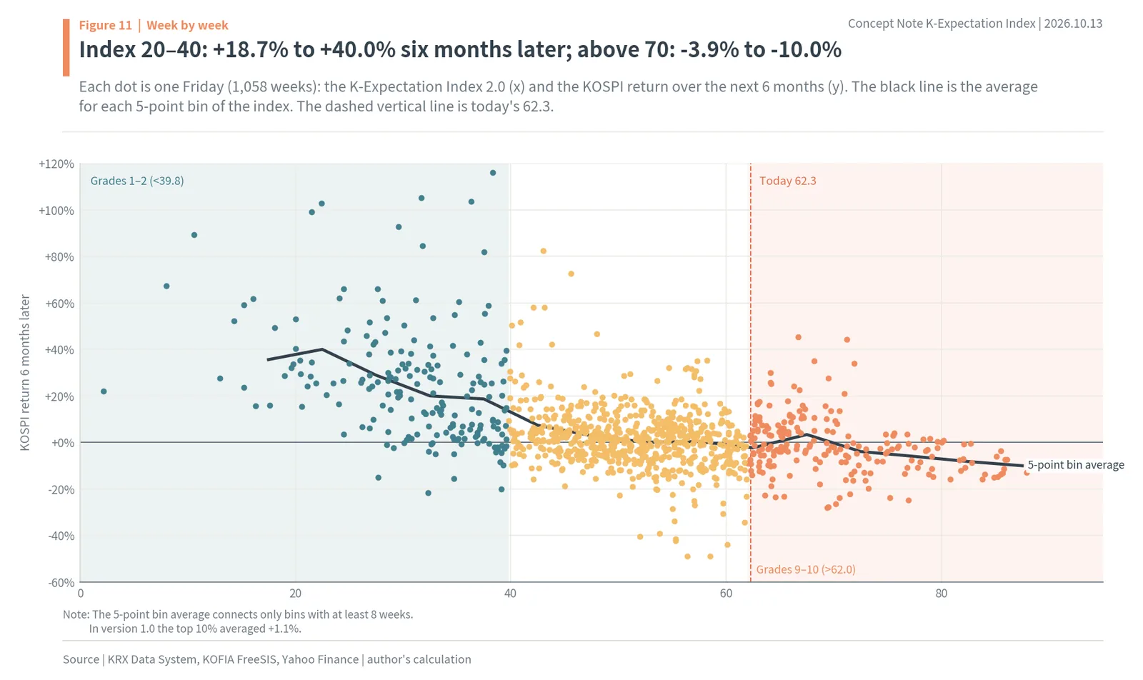
Figure 11 plots each Friday’s K-Expectation Index 2.0 (horizontal) against the KOSPI return over the next 6 months (vertical), 1,058 weeks in all. The dots form a band that slopes down to the right. Averaging later returns in 5-point bins of the index and connecting them, the bins from 20 to 40 averaged +18.7% to +40.0%, the bins from 45 to 60 +0.1% to +2.9%, and the bins above 70 -3.9% to -10.0%. In version 1.0 the top 10% averaged +1.1%; in version 2.0, above 70, each higher bin is lower than the one before. Most dots below 40 sit above the 0% line, and many dots above 62 cluster below it. Even at the same index value, later returns are widely scattered. The index is not a tool that predicts the future as a single number; it is a tool that tells you which way the odds lean. Even in the bottom zone, 15% of days were down six months later, and even in the overheated zone, 36% were up. So the index is better used as a guide for raising and trimming stock exposure than as a signal to buy or sell everything at once.

KOSPI peaks and bottoms since 2006: bottoms at 39.5 or lower, peaks at 47.6 or higher

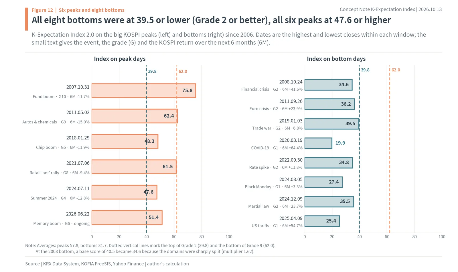
All eight bottoms were within Grade 2

Averages alone do not show how the index behaved at actual turning points. So the author picked the six big KOSPI peaks and eight big bottoms since 2006 and looked at the index on those days (Figure 12). The dates were not hand-picked: they are the highest and lowest closes within each window. The bottoms were October 24, 2008 (global financial crisis, 938.75), September 26, 2011 (European debt crisis, 1,652.71), January 3, 2019 (US-China trade war, 1,993.70), March 19, 2020 (COVID-19, 1,457.64), September 30, 2022 (rate spike, 2,155.49), August 5, 2024 (global “Black Monday” sell-off, 2,441.55), December 9, 2024 (martial law shock, 2,360.58) and April 9, 2025 (US tariffs, 2,293.70).

At the eight bottoms the K-Expectation Index 2.0 averaged 31.7, and even the highest was 39.5 (January 3, 2019), so all were within Grade 2 (below 39.8). March 19, 2020 (19.9), April 9, 2025 (25.4) and August 5, 2024 (27.4) were Grade 1. The 6-month returns that followed were +64.4% in 2020, +54.7% in 2025 and +3.3% after August 2024, and the 1-year returns were +106.4%, +171.1% and +29.1%. In version 1.0, October 24, 2008 (40.5) and January 3, 2019 (41.5) fell outside the bottom bin. In version 2.0 they came in at 34.6 and 39.5. Both days had a base score near 40, but the domains were sharply split, giving multipliers of 1.62 and 1.24. At the 2008 bottom, a price score of 0.1 and a fear score of 0.0 pointed to a bottom, while debt (67.3) and heat (68.7) stayed high.

All six peaks were at 47.6 or higher

The peaks were October 31, 2007 (fund boom, 2,064.85), May 2, 2011 (the autos, chemicals and refiners rally, 2,228.96), January 29, 2018 (chip boom, 2,598.19), July 6, 2021 (the “Donghak ant” retail wave, 3,305.21), July 11, 2024 (2,891.35) and June 22, 2026 (memory chip surge, 9,114.55). At the six peaks the index averaged 57.8, and even the lowest was 47.6 (July 11, 2024). October 31, 2007 read 75.8, Grade 10, and was followed by -11.7% over 6 months and -42.8% over 1 year. May 2, 2011 read 62.4, Grade 9, and July 6, 2021 read 61.5, Grade 8; the 1-year returns that followed were -10.5% and -29.9%.

There is a gap of more than 26 points between the bottom average (31.7) and the peak average (57.8), and the two groups do not overlap. The highest bottom was 39.5 and the lowest peak was 47.6. The index does not hit its high exactly on peak days, but it puts peaks and bottoms in different zones.

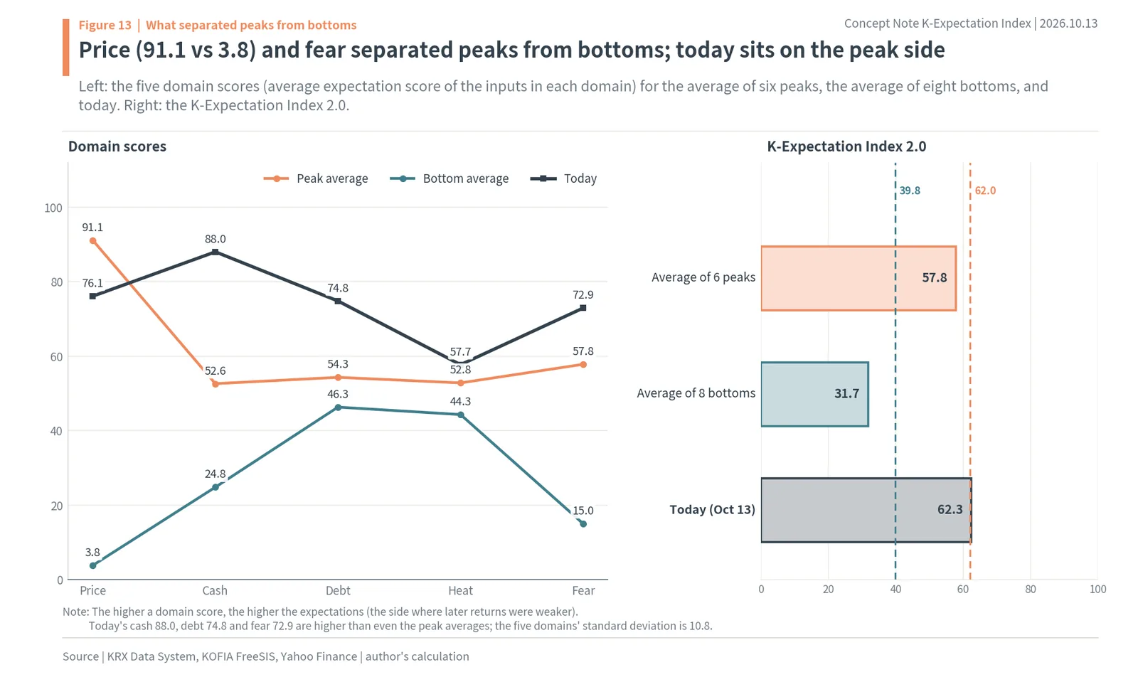
Price and fear separated peaks from bottoms

Averaging the five domain scores at peaks and at bottoms shows what separated them (Figure 13). The price domain split the most, averaging 91.1 at peaks and 3.8 at bottoms: at peaks PBR was near its highest of the prior 3 years, and at bottoms near its lowest. The fear domain averaged 57.8 at peaks and 15.0 at bottoms; at bottoms the VIX spiked and the won weakened, pulling the fear score down. The cash domain averaged 52.6 at peaks and 24.8 at bottoms, because at bottoms plenty of deposits were left relative to market cap. The debt domain (54.3 at peaks, 46.3 at bottoms) and the heat domain (52.8 at peaks, 44.3 at bottoms) differed little. Near bottoms, debt shrinks through forced selling, which pushes up the margin loan growth input’s score, and trading piles up relative to deposits, which pushes up the turnover input’s score. So at bottoms a split shape, with price and fear low and debt and heat less low, shows up often, and the dispersion multiplier reads that shape as a stronger bottom signal.

Today’s (October 13) domain scores are price 76.1, cash 88.0, debt 74.8, heat 57.7 and fear 72.9. Price is below the peak average (91.1) but far from the bottom average (3.8). Cash (88.0) and debt (74.8) are above even the peak averages, and fear (72.9) is also above the peak average (57.8). The five domains are evenly high, so the dispersion is a small 10.8, which is why the multiplier pressed the index down to 62.3. Today’s profile is much closer to a peak than to a bottom.

KOSPI in 2026: the index went from 2.2 in March to 51.4 at the June peak and 62.3 now

While KOSPI nearly tripled, the index sat on the bottom side

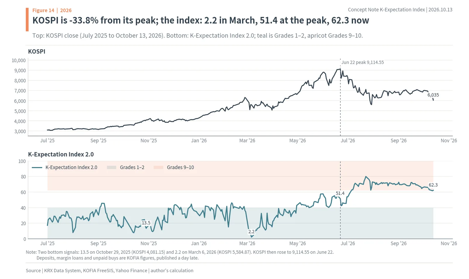
2026 is the most extreme year on which to test this index. The KOSPI nearly tripled in just over a year, from 3,089.65 on July 1, 2025 to 9,114.55 on June 22, 2026, and then fell 33.8% to 6,035.35 on October 13. Figure 14 plots the KOSPI and the K-Expectation Index 2.0 over this period. While the KOSPI was rising most steeply, the index actually stayed on the bottom side. It was 17.3 on July 1, 2025, Grade 1.

Two bottom signals: October 2025 and March 2026

Twice during the bull market the index fell into Grade 1. The first was October 29, 2025. The KOSPI was at 4,081.15 and PBR at 1.37x was the most expensive of the prior 3 years (price score 100.0). But deposits were growing fast at KRW 85.9tn (cash 9.3), trading was not heavy relative to deposits (heat 15.7), and USD/KRW at 1,426.0 meant a weak won (fear 30.8). The base score was 29.0, and with only price high and the rest low, the domain dispersion was a large 36.5. A multiplier of 1.74 strengthened the bottom signal, and the index was 13.5. The KOSPI more than doubled over the next eight months.

The second was March 2026. On March 4 the KOSPI fell 12.1% from the previous day to 5,093.54; the VIX reached 29.49 on March 6, and USD/KRW was 1,479.5. The fear domain’s score fell to 1.1. Deposits had piled up to KRW 130.0tn, large relative to market cap, so the cash domain scored just 0.4. The price domain was still expensive at 98.9. A base score of 25.0 combined with a dispersion of 40.2 put the index at 2.2 on March 6, the lowest value since 2006. The KOSPI then rose 63.2%, from 5,584.87 on March 6 to 9,114.55 on June 22. In the middle of a bull market, the index read a day when fear and cash swung to extremes as its strongest bottom signal.

The peak day read 51.4, in the neutral zone

On June 22, the day of the peak, the domain scores were price 99.5, cash 68.3, debt 43.1, heat 53.8 and fear 18.3. Price was the most expensive of the prior 3 years. But USD/KRW at 1,531.3 (1,506.8 to 1,554.5 throughout June) meant a weak won that kept the fear side low, and fast-growing debt and a low margin loans ÷ deposits ratio (29.1%) kept the debt side low. The base score was 51.0 and the multiplier 1.44, so the index was 51.4, Grade 6. PBR on June 22 was 2.59x.

After the peak, money left and the index rose

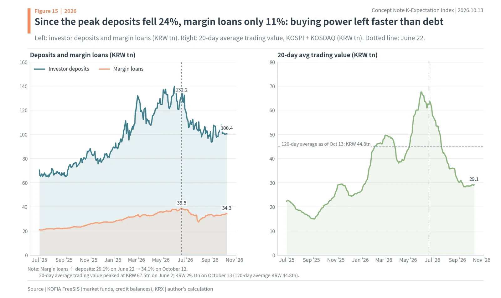
After June 22, as the KOSPI fell, the index rose. On July 16 it entered Grade 10 at 71.2 with the KOSPI at 6,820.60, and it was 65.8 on September 30 and 62.3 on October 13. Figure 15 shows how money moved in the meantime. Investor deposits fell 24%, from KRW 132.2tn on June 22 to KRW 100.4tn on October 12. Margin loans fell 11% over the same period, from KRW 38.5tn to KRW 34.3tn. With deposits shrinking more than twice as fast as debt, margin loans ÷ deposits rose from 29.1% to 34.1%. The buying money left while the debt stayed. The 20-day average trading value (KOSPI plus KOSDAQ) peaked at KRW 67.5tn (about $50.4bn) on June 2 and shrank to KRW 29.1tn (about $21.7bn) on October 13. As trading cooled, the heat domain’s trading surge input reached an expectation score of 97.6. This is not panic selling with exploding volume, but quiet selling on the way out.

A stronger won and a calm US market: no fear

The fear domain also pushed the index up. USD/KRW came down from 1,531.3 on June 22 to 1,338.8 on October 13. In this index a stronger won reads as “no fear outside Korea,” because the tendency of KOSPI bought on a weak won to do well a year later (rank correlation +0.34) goes in flipped. The US VIX actually fell, from 17.28 on June 22 to 15.33 on October 13. Only the KOSPI dropped, while the US market stayed calm. So today’s fear domain score is 72.9, far above the 18.3 of the peak day.

2026 also shows why the VKOSPI was left out of the formula (Figure 16, right). The VKOSPI averaged 58.9 from January to June 2026, while the KOSPI was rising, and from March to June it never fell below 48.51. On June 22, the day of the peak, it was 87.36. In a market that moves several percent a day, volatility runs high even on the way up, so the VKOSPI reads high. On October 13 the VKOSPI was 48.53, lower than on the peak day. Read on its own, the VKOSPI says investors are less scared now than at the peak. The US VIX and USD/KRW are removed from the KOSPI’s own swings, so they show more cleanly whether fear is coming from outside Korea.

Today’s decline is a quiet exit

The 2026 story fits in one line. On days when money poured in and fear spiked, the index sat on the bottom side even though stocks were expensive; once money started leaving, the index rose even as prices fell. This year’s median domain dispersion was 30.0, and today it is 10.8: the five domains have bunched together on the high side. That is why the multiplier pressed the index down to 62.3, but it is still at the threshold of the overheated zone. At past bottoms, trading exploded, debt was cut all at once by forced selling, and the won weakened or the VIX spiked. None of that has happened yet, which is why the index is high.

Today’s ten inputs: base score 73.8, dispersion multiplier 0.516, index 62.3

Nine of the ten are on the high-expectation side

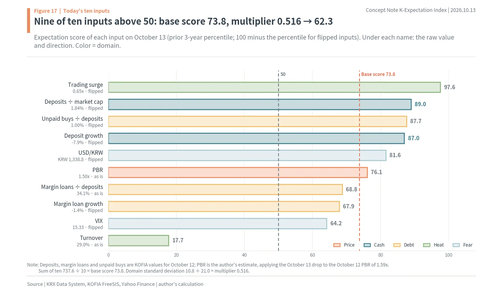
Figure 17 shows the raw values and expectation scores of the ten inputs as of October 13. Investor deposits, margin loans and unpaid purchases are KOFIA’s October 12 values, because KOFIA publishes them a day late; the rest are October 13 values. Nine of the ten inputs have an expectation score above 50.

The highest is trading surge (97.6). The 20-day average trading value of KRW 29.1tn divided by the 120-day average of KRW 44.8tn is 0.65x, in the bottom 2.4% of the prior 3 years. There were almost no days in the past 3 years when trading had cooled this much. Next is deposits ÷ market cap (89.0). Deposits of KRW 100.4tn divided by the combined KOSPI and KOSDAQ market cap of KRW 5,451tn (about $4.07tn) is 1.84%, right against the prior 3 years’ 10% mark (1.81%). Unpaid purchases ÷ deposits (87.7) is 1.00%, on the low side of the 3 years, so there is no trace of panic selling where buyers piled in beyond what they could settle. Deposit growth (87.0) is -7.9%, from KRW 109.0tn 60 trading days ago to KRW 100.4tn. USD/KRW (81.6) is 1,338.8, in the bottom 18% of the prior 3 years, on the strong-won side.

Price is a PBR of 1.50x (76.1). This is the author’s estimate, applying the October 13 index decline to KRX’s published October 12 PBR of 1.59x. The prior 3 years’ median is 0.99x, the 75% mark 1.40x and the 90% mark 1.95x. Because the 3-year window includes 2023–2025, when PBR hovered around 1x, 1.50x reads as well above that. Margin loans ÷ deposits (68.8) is 34.1%, close to the 3-year 75% mark (34.8%). Margin loan growth (67.9) is -1.4% over 60 trading days: debt has barely shrunk. The VIX (64.2) is 15.33, a little below its 3-year median (16.35).

Only turnover (17.7) has a low expectation score. The 20-day average trading value of KRW 29.1tn divided by deposits of KRW 100.4tn is 29.0%, so there is little trading relative to the cash in accounts. The ten expectation scores add up to 737.6, and divided by 10 the base score is 73.8.

The dispersion multiplier is then applied to this base score. The domain scores are price 76.1, cash 88.0, debt 74.8, heat 57.7 and fear 72.9, all five gathered between 57 and 88. The dispersion is 10.8, just over half the median since 2006 (21.0), and the multiplier is 0.516. So the K-Expectation Index 2.0 is 50 + 23.8 × 0.516 = 62.3, in the top 19.6% of all days since 2006, Grade 9. Days bought in Grade 9 averaged 0.0% six months later (47% up), below the post-2006 average (+4.1%).

The dashboard view

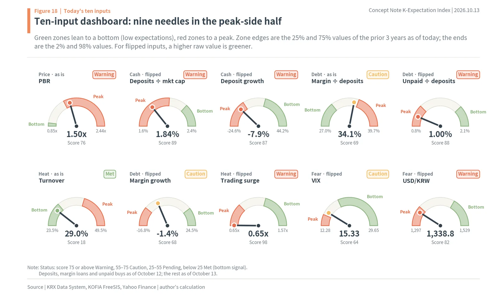
Figure 18 draws the ten inputs as gauges. A needle in the green zone leans to a bottom (low expectations); in the red zone, to a peak (high expectations). The zone edges are the 25% and 75% values of the prior 3 years as of today. For flipped inputs, a higher raw value is greener. For example, USD/KRW is green above 1,451 (the 3-year 75% mark) and red below 1,351 (the 25% mark), and today’s 1,338.8 is in the red zone. Deposits ÷ market cap is green above 2.20% and red below 2.03%, and today’s 1.84% is red. Margin loans ÷ deposits works the other way: green below 30.6% and red above 34.8%, and today’s 34.1% sits at the red end of the middle zone.

This dashboard can be checked every day. As a bottom approaches, the inputs in the red zone cross over toward green one by one. As shown above, at the past eight bottoms the average domain scores were price 3.8, fear 15.0 and cash 24.8. Whether the needles for these three domains cross into the green zone is the first thing to watch.

What it takes to reach a bottom grade: a 20% drop alone gives 58.2 (Grade 8)

Lower prices alone: Grade 8

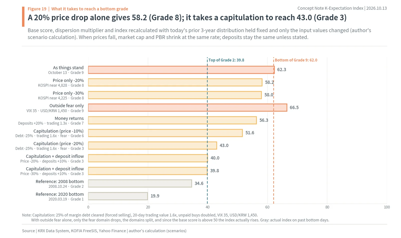
What would have to change for an index at 62.3 (Grade 9) today to reach the bottom zone (Grades 1 and 2, below 39.8)? The author held today’s prior 3-year distribution fixed, changed only the inputs’ values and recalculated the base score and the dispersion multiplier (author’s calculation, Figure 19). When prices fall, market cap and PBR were assumed to shrink at the same rate, with the amount of deposits unchanged unless set separately.

If prices fall another 20% with everything else unchanged, the index is 58.2, Grade 8. In KOSPI terms that is around 4,828. As market cap shrinks, deposits ÷ market cap rises to 2.30% and that input’s expectation score drops from 89.0 to 7, bringing the base score to 64.8, but PBR at 1.20x is still on the high side of the 3-year window (68), and with the other inputs unchanged the index stays in the high zone. Even a 30% price drop (KOSPI around 4,225) gives 58.0. If money comes back instead, with prices unchanged, deposits up 20% and trading value at 1.3x, the index is 56.3, Grade 7.

Outside fear on its own moves differently. If the VIX jumps to 35 and USD/KRW reaches 1,450, the two fear inputs drop to 1 and 26 and the base score falls to 61.8. But with the fear domain dropping alone, the five domains split and the dispersion grows (multiplier 1.40), and since the base score is still above 50, the index actually rises to 66.5. As shown in the formula section, days with a high base score and split domains had poor 6-month returns in both decades (-7.2% and -4.2%). Fear spiking outside Korea while the other domains stay high is not a bottom signal.

Capitulation: Grade 3, and with deposits flowing back, the Grade 2 threshold

The author then modeled several things happening at once, as at past bottoms: a “capitulation” bundle in which prices fall 20%, a quarter of margin debt is cleared through forced selling, the 20-day average trading value rises 1.6x, unpaid purchases double, the VIX hits 35 and USD/KRW reaches 1,450. The base score is then 44.1 and the multiplier 1.18, so the index is 43.0, Grade 3. With the same capitulation plus a 10% inflow of deposits, that is, money from panic sales piling up in accounts, it is 40.0, and with a 30% price drop it is 39.8, reaching the Grade 2 threshold. That is the same height as the eight big bottoms in the past (19.9 to 39.5).

Two inputs explain why even a capitulation does not take the index very low. One is PBR. The prior 3 years include 2023–2025, when PBR hovered around 1x, so even if the KOSPI falls another 20% to 30% and PBR drops to 1.05x to 1.20x, it still reads as expensive within the 3-year window (60 to 68). The other is margin loan growth. When debt is cut all at once by forced selling, this flipped input gets an expectation score of 100, reflecting the past average that returns were weak after debt shrank fast. So for the index to reach Grade 1, fear and cash have to swing to extremes as in March 2026, or time has to pass until the PBR-around-1x years drop out of the 3-year window. On March 6, 2026, fear at 1.1 and cash at 0.4 pulled the base score down to 25.0, and a dispersion of 40.2 (multiplier 1.92) strengthened the signal, taking the index to 2.2.

The author’s view

The author reads today not as a bottom where expectations have broken, but as a stretch where the buyers are running out. Prices have come down 33.8% from the peak, but money is leaving quietly, debt has shrunk less, and the outside world is calm. The index is 62.3, Grade 9, at the threshold of the overheated zone, and days bought in Grades 9 and 10 averaged -2.4% six months later, with only 36% up. A bottom signal does not come from lower prices; it comes when debt is cleared through forced selling, the VIX and USD/KRW point to fear, and deposits build up again. In terms of this index’s inputs, that signal is margin loans ÷ deposits falling below 30%, USD/KRW rising above 1,450, and the 20-day average trading value climbing back above the 120-day average.

How to calculate the K-Expectation Index 2.0 yourself in six steps

Every input is public data

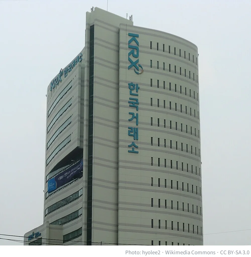
Every input to the K-Expectation Index 2.0 is a number published every day. KOSPI and KOSDAQ index levels and market caps, trading value and KOSPI PBR are posted daily by the Korea Exchange on its Data System. Figure 20 shows the Korea Exchange building in Dong-gu, Busan, photographed in March 2012. Investor deposits, unpaid purchases and margin loans are posted to KOFIA FreeSIS a day late, and the US VIX and USD/KRW are available from quote sites such as Yahoo Finance.

Six steps

Figure 21 draws the calculation as a six-step staircase. First, download the data. Calculating 3-year percentiles requires at least the prior 3 years, roughly 756 trading days, of data, and adding the extra 120 days needed for growth rates and moving averages, it is easiest to download four years. KOFIA data are posted a day late, so today’s index uses yesterday’s values.

Second, calculate the ten raw values. PBR is used as is. Margin loans ÷ deposits divides total margin loans (KOSPI plus KOSDAQ) by investor deposits. Unpaid purchases ÷ deposits divides the 5-day average of unpaid purchases by deposits. Margin loan growth divides today’s margin loans by the value 60 trading days earlier and subtracts 1. Deposits ÷ market cap divides deposits by the combined KOSPI and KOSDAQ market cap. Deposit growth divides today’s deposits by the value 60 trading days earlier and subtracts 1. Turnover divides the 20-day average of combined KOSPI and KOSDAQ trading value by deposits. Trading surge divides the 20-day average of the same trading value by its 120-day average. The VIX and USD/KRW are used as is.

Third, convert each value into a 3-year percentile and set its direction: count what percentage of the prior 756 trading days, including today, had a value below today’s. In Excel, the PERCENTRANK function does this. Three inputs, PBR, margin loans ÷ deposits and turnover, use the percentile as is; the other seven (unpaid purchases ÷ deposits, margin loan growth, deposits ÷ market cap, deposit growth, trading surge, VIX and USD/KRW) use 100 minus the percentile. Fourth, add the ten expectation scores and divide by 10 to get the base score. Fifth, take the standard deviation of the five domain scores (price is PBR; cash is the average of its two inputs; debt the average of its three; heat and fear the averages of their two) and divide it by 21.0 to get the dispersion multiplier. In Excel that is the STDEV.S function. Sixth, calculate 50 + (base score – 50) × dispersion multiplier, clip it to the ends if it falls outside 0 to 100, and assign the grade using the cutoffs (32.7, 39.8, 44.7, 48.2, 51.4, 54.3, 57.6, 62.0, 68.3).

How to read and use it

Read the index by zone. Grades 1 and 2 (below 39.8) are the bottom zone, and Grades 9 and 10 (above 62.0) are overheated. As shown earlier, later returns are widely scattered even within a zone, so this index works better as a scale for raising and lowering stock exposure than as a button for buying or selling everything at once. For example, hold more stocks than usual in the bottom zone and fewer than usual in the overheated zone.

The index does not swing much from day to day. Six of the ten inputs are 20- to 120-day averages or 60-day growth rates, so they move slowly, and the 3-year window changes by only one day each day. On October 12 the index was 61.7 and on October 13 62.3: on a day when the KOSPI fell more than 5%, the index moved 0.6 points. So checking it once a week, on Friday’s value, is enough. Because all the inputs are market-wide numbers, the index does not value individual stocks. When expectations for the market as a whole are overheated, most stocks wobble together, so use it as the backdrop for timing trades in your own stocks: in the bottom zone, bring forward purchases you have been putting off; in the overheated zone, hold off on new purchases and trim the stocks that have risen the most first.

Data and methods: KRX, KOFIA and Yahoo Finance data and the author’s calculations

Data and periods

KOSPI and KOSDAQ index closes, highs, lows, trading value and market caps, and the VKOSPI, were downloaded from the KRX Data System’s individual index trend pages for January 2, 2003 to October 13, 2026 (KOSPI 1/001, KOSDAQ 2/001, VKOSPI 1/300). KOSPI PER and PBR come from the KRX index PER/PBR/dividend yield pages, from January 2, 2004. KRX still showed the October 13 PBR as 0, so it was estimated at 1.50x by applying the October 13 KOSPI decline (-5.46%) to the October 12 PBR of 1.59x. Net buying by investor type is from KRX’s KOSPI trading by investor type (net buying value). Investor deposits, unpaid purchases and forced selling come from KOFIA FreeSIS’s market funds trend (from June 1998), and margin loans from its credit balance trend (from January 1998), in millions of won. KOFIA data are published a day late, so the dates were aligned to trading days and gaps were filled with the previous value. The US VIX and USD/KRW are Yahoo Finance daily closes (^VIX, KRW=X), aligned to Korean trading days using the previous value.

The index was calculated from January 2, 2006 to October 13, 2026. The first 3-year percentiles need earlier data, so 2003–2005 data were used only for percentile calculation. Percentiles were calculated in a trailing 756-trading-day window, and a value was produced only when the window held at least 378 days of data. Ties were given their average rank.

Target and testing

Later returns are log returns of the KOSPI close 60, 120 and 250 trading days ahead. The average returns shown in this report are averages of log returns converted back to percent, and the share up is the share of days with a later return above zero. The target used to choose formulas is the average of the three horizons’ log returns, each standardized to a mean of 0 and a standard deviation of 1. Rank correlation is Spearman’s rank correlation coefficient. Daily later returns overlap (today’s and tomorrow’s 6-month returns cover almost the same period), so treating them as 5,000 observations would overstate statistical significance. That is why this report uses working separately in two decades as its standard instead of significance.

The two decades are January 2006 to December 2014 (first) and January 2016 to October 2026 (second). 2015 was left empty so that later returns from the first period do not spill into the second. Each input’s direction (as is or flipped) was set by the sign of its rank correlation with the three-horizon target over 2006–2026 as a whole; the ten chosen inputs had the same sign in both decades, so their direction is the same whichever period sets it. The fitted formulas (see “The best-fit formula got it backwards”) used non-negative least squares (scipy nnls) to fit the direction-adjusted expectation scores, minus their mean, to the sign-reversed target, and the weights were rescaled to sum to 1. The “choose from one decade only” test split the training decade again at its midpoint and picked inputs with the same sign in both halves and a weaker-half rank correlation of at least 0.05.

Calculating version 2.0

The base score is the simple average of the ten expectation scores (the same as version 1.0). The domain scores are the average expectation scores within price (PBR), cash (deposits ÷ market cap, deposit growth), debt (margin loans ÷ deposits, unpaid purchases ÷ deposits, margin loan growth), heat (turnover, trading surge) and fear (VIX, USD/KRW). Dispersion is the sample standard deviation (dividing by n-1) of the five domain scores, and the reference value of 21.0 is the median dispersion from January 2006 to October 13, 2026. K-Expectation Index 2.0 = 50 + (base score – 50) × (dispersion ÷ 21.0), set to 0 if below 0 and 100 if above 100 (no day since 2006 actually hit either end). The multiplier-strength test in the formula section used 50 + (base score – 50) × (1 + c × (dispersion ÷ 21.0 – 1)) with c set to 0, 0.5, 1.0 and 1.5; version 2.0 is c = 1.0.

The aligned-versus-split table in the formula section took days with a base score in the bottom 20% (below 39.3) or the top 20% (above 61.6) and split them by whether dispersion was below or above that decade’s median (20.8 in 2006–2014, 21.0 in 2016–2026). The devices tested and dropped were defined as follows. A score curve converts an expectation score x into 50 + 50 × sign(d) × |d|^γ, where d = (x – 50) ÷ 50 (γ = 0.6, 1.5, 2, 3); the step score table gives 0, 20, 40, 50, 60, 80 or 100 points to percentile bands of 0–10, 10–25, 25–40, 40–60, 60–75, 75–90 and 90–100. A “fear peak” is a day when the VIX and USD/KRW percentiles are both 85 or higher, and “capitulation confirmed” is a day when either one is 85 or higher and the trading surge percentile is 80 or higher. A combined signal’s effect (in percentage points) is the difference in 6-month returns between days with the signal on and off within each of five bins of the version 1.0 score, averaged with the number of signal days as weights.

Zones, events and scenario calculations

The ten grades’ cutoffs are the 10%, 20%, … 90% quantiles of the K-Expectation Index 2.0 from January 2006 to October 13, 2026 (32.7, 39.8, 44.7, 48.2, 51.4, 54.3, 57.6, 62.0, 68.3), and the five zones pair the grades two by two (cutoffs 39.8, 48.2, 54.3, 62.0). Today’s 62.3 was placed in the same distribution: in the top 19.6%. Version 1.0’s (the base score’s) five-bin cutoffs are 39.3, 47.9, 54.5 and 61.6, and the formula section’s “base score bottom and top 20%” used these cutoffs. Peak and bottom dates are the highest and lowest closes within windows set by the author. The peak windows are January 2007 to June 2008, January to August 2011, October 2017 to June 2018, 2021, January to September 2024 and 2026; the bottom windows are 2008, August to December 2011, July 2018 to January 2019, January to June 2020, 2022, August 1 to 10, 2024, November 2024 to January 2025 and March to May 2025. A domain score is the average expectation score of the inputs in that domain.

The scenario calculations held fixed the distribution of raw values over the 756 trading days to today, recalculated each expectation score from where the changed raw value falls in that distribution, and then recalculated the base score, the domain dispersion, the dispersion multiplier and the index in turn. When prices fall x%, the KOSPI and KOSDAQ market caps and PBR shrink at the same rate, and deposits stay the same unless set separately. Clearing debt reduced the amount of margin loans (the value 60 trading days earlier stays the same, so margin loan growth changes too); for trading value, the 20-day average was changed and the 120-day average by 20/120 of the difference. For unpaid purchases, the 5-day average was changed. In reality the 3-year window moves as time passes, so the scenarios are a yardstick for where the index would land if these things happened against today’s distribution.

Photos

Figure 1 is a photo by TurnOnTheNight on Wikimedia Commons (taken May 1, 2024, CC BY-SA 4.0), and Figure 20 is a photo by hyolee2 (taken March 7, 2012, CC BY-SA 3.0), cropped to the upper part of the building. The captions follow the file descriptions on Wikimedia Commons.

2026 figures

Deposits (KRW 132.2tn to KRW 100.4tn) and margin loans (KRW 38.5tn to KRW 34.3tn) on June 22 and October 12 are KOFIA daily values; deposits peaked for 2026 at KRW 139.7tn on June 4, and margin loans at KRW 38.6tn on June 24. The 20-day average trading value peaked at KRW 67.5tn on June 2. The VKOSPI’s 87.36 (June 22) and 48.53 (October 13) are KRX values; the VIX’s 17.28 and 15.33 and USD/KRW’s 1,531.3 and 1,338.8 are Yahoo Finance values.

Korean stock market sentiment index FAQ

Sources

1. Korea Exchange (KRX) Data System via pykrx, KOSPI and KOSDAQ index price trends (close, trading value, market cap) and the KOSPI 200 volatility index (VKOSPI), 2003.01.02 to 2026.10.13 (link)
2. KRX Data System via pykrx, KOSPI PER, PBR and dividend yield, 2004.01.02 to 2026.10.13 (link)
3. KRX Data System via pykrx, KOSPI trading by investor type (net buying value), 2004.01.02 to 2026.10.13 (link)
4. Korea Financial Investment Association (KOFIA) FreeSIS, market funds trend (investor deposits, unpaid purchases, forced selling), 1998.06.18 to 2026.10.12, retrieved 2026.10.13 (link)
5. KOFIA FreeSIS, credit balance trend (margin loans, stock borrowing on margin), 1998.01.30 to 2026.10.12, retrieved 2026.10.13 (link)
6. Yahoo Finance, US VIX (^VIX) and USD/KRW (KRW=X) daily closes, 2002.01.02 to 2026.10.13 (link)
7. The 21 candidates’ percentiles, the two-decade test, the non-negative least squares weights, the dispersion multiplier and grade cutoffs, forward returns by grade and zone, the peak and bottom dates and the scenario calculations are all the author’s calculations
8. Photo (Figure 1 and featured image): TurnOnTheNight, “Cityscape of Yeouido skyscrapers and Hangang Railway Bridge” (link), CC BY-SA 4.0 (link), via Wikimedia Commons
9. Photo (Figure 20): hyolee2, “Korea exchange.JPG” (link), CC BY-SA 3.0 (link), via Wikimedia Commons